|
VCSBeam
|
|
VCSBeam
|
There are three coordinate systems in use throughout VCSBeam:
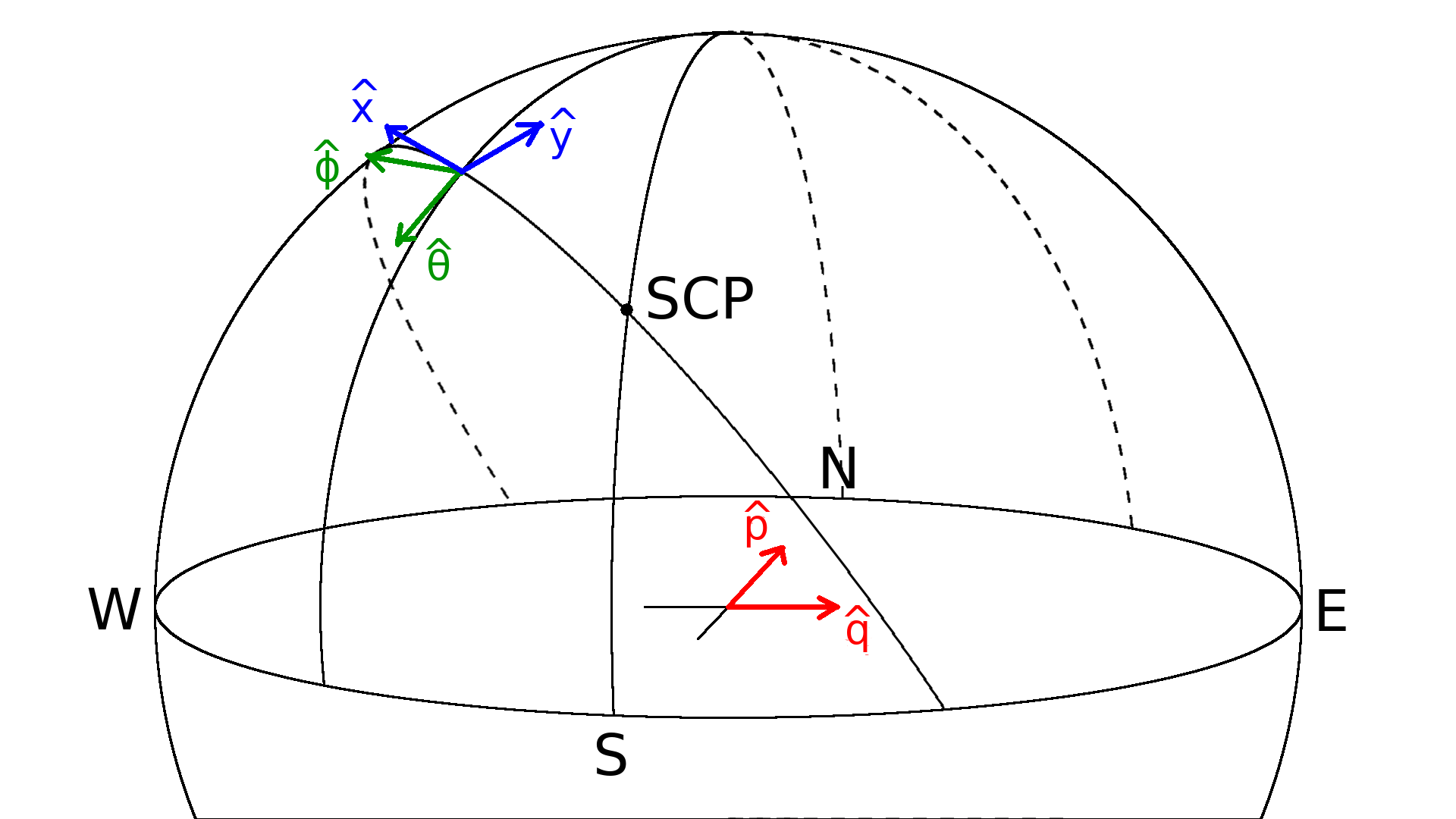
This is a Cartesian coordinate system aligned with local (ground) compass directions. Positive \(p\) points towards local North, and positive \(q\) towards local East. The \(P\) polarisation refers to the physical set of dipoles parallel to the N-S line; the \(Q\) polarisation, to the E-W line.
This is a spherical coordinate system defined with respect to a local observer. \(\theta\) is the zenith angle, i.e. a colatitude, with zenith itself therefore defined as \(\theta = 0\) and the horizon as \(\theta = \pi/2\). \(\phi\) is the azimuth, and we define \(\phi = 0\) in the North direction, with positive azimuth moving clockwise as viewed from above (i.e. N→E→S→W→N). Moreover, the elevation is denoted by the symbol \(\tilde{\theta}\), and is related to the zenith angle by
\[ \tilde{\theta} = \frac{\pi}{2} - \theta. \]
This is a spherical coordinate system defined with respect to the celestial sphere. \(x\) is the declination (Dec) and \(y\) is the right ascension (RA).
All coordinate transformations can be effected by applying the appropriate Jacobian matrix for the desired transformation. In this documentation, a boldface \({\bf P}\) will always be used to denote transformation matrices. For general coordinates \((a,b)\) and \((c,d)\),
\[ {\bf P}_{(a,b)\rightarrow(c,d)} \equiv \begin{bmatrix} P_{ca} & P_{cb} \\ P_{da} & P_{db} \end{bmatrix} \equiv \begin{bmatrix} \frac{\partial c}{\partial a} & \frac{\partial c}{\partial b} \\[5 pt] \frac{\partial d}{\partial a} & \frac{\partial d}{\partial b} \end{bmatrix} \]
Among these, the only transformation that is explicitly used in VCSBeam is the transformation between local sky coordinates and celestial sky coordinates, which is a single rotation within the sky plane by the parallactic angle.
The parallactic angle correction is a transformation between local sky coordinates and celestial sky coordinates. The parallactic angle itself, \(\chi\), is defined as the position angle of local zenith with respect to the North Celestial Pole as subtended at a given source, illustrated in the following figure.

The transformation \((x,y)\rightarrow(\theta,\phi)\) is therefore a counterclockwise rotation by \(\pi - \chi\). (A counterclockwise rotation of a given vector is equivalent to a clockwise rotation of the coordinate axes.) This is the rotation
\[ {\bf P}_\text{pa} = \begin{bmatrix} P_{\theta x} & P_{\theta y} \\ P_{\phi x} & P_{\phi y} \end{bmatrix} = \begin{bmatrix} \cos\left(\pi - \chi\right) & -\sin\left(\pi - \chi\right) \\ \sin\left(\pi - \chi\right) & \cos\left(\pi - \chi\right) \end{bmatrix} = \begin{bmatrix} -\cos\chi & -\sin\chi \\ \sin\chi & -\cos\chi \end{bmatrix}. \]
In VCSBeam, the parallactic angle is calculated (via the function palPa) in the Starlink/pal library by the spherical triangle identity
\[ \tan \chi = \frac{\cos \lambda \sin H}{\sin\lambda \cos x - \cos \lambda \sin x \cos H}, \]
where \(\lambda\) is the latitude of the observer, \(H\) is the hour angle of the source, and \(x\) is the declination. The latitude of the MWA is \(\lambda_\text{MWA} = -0.4660608448386394\) rad, defined in the mwalib library.
All data are functions of time (t), frequency (f), antenna (a), and/or polarisation (p). Accordingly, the size of data arrays are expressed in terms of \(N_t\), \(N_f\), \(N_a\), and \(N_p\). The order of the dimensions indicates the layout of the data arrays in memory, with the first dimension being the slowest changing dimension, and so on until the last dimension, which is the fastest changing. For example, the instrumental calibration matrices ( \({\bf D}\)) have dimensions
\[ N_a \times N_f \times N_p \times N_p, \]
and a single element is specified with the index notation, \(D_{a,f,p_1,p_2}\). Jones vectors, indicated with a lower case Latin letter in bold, include a polarisation dimension implicitly, e.g.
\[ {\bf e} = \begin{bmatrix} e_x \\ e_y \end{bmatrix}, \]
where \(x\) and \(y\) are examples of a specific polarisation basis. Similary, Jones matrices, represented with bold uppercase Latin letters, have two implied polarisation dimensions, e.g.
\[ {\bf J} = \begin{bmatrix} J_{xx} & J_{xy} \\ J_{yx} & J_{yy} \end{bmatrix}. \]
The exception to the above system is the data layout of the legacy recombined format, in which the combinations of antennas and polarisations are ordered in a "mixed" way, so that it cannot be said that either antennas or polarisations change faster than the other. For this case, we describe a particular antenna-polarisation combination as an "input", and denote it with the subscript \(i\), with \(N_i = N_a \times N_p\) (without the implied hierarchical ordering).
Full Stokes parameters are the set \(\{I, Q, U, V\}\). Accordingly, an array containing these "post-detection" products may include the dimension \(N_s\), which always equals exactly 4.
Each MWA tile contains \(N_d = 16\) dipoles.
Multiple pointings can also be processed simultaneously, and some output arrays therefore include dimension \(N_b\).
The complete list, in alphabetical order of subscripts, is
| Symbol | Description | Typical values |
|---|---|---|
| \(N_a\) | Number of tiles/antennas | 128 |
| \(N_b\) | Number of beams/pointings | 1 |
| \(N_d\) | Number of dipoles per tile | 16 |
| \(N_f\) | Number of frequencies per coarse channel | 128 |
| \(N_p\) | Number of polarisations | 2 |
| \(N_s\) | Number of Stokes parameters | 4 |
| \(N_t\) | Number of timesteps/samples per second | 10000 |
| Document | ||||||
|---|---|---|---|---|---|---|
| This document | \(p\) | \(q\) | \(\theta\) | \(\phi\) | \(x\) | \(y\) |
| MWA metafits files | Y | X | - | - | - | - |
| Document | |||
|---|---|---|---|
| This document | \({\bf J}\) | \({\bf D}\) | \({\bf B}\) |
| Sokolowski et al., (2017) | \({\bf J}\) | \({\bf G}\) | \({\bf E}\) |
| Ord et al., (2019) | \({\bf J}\) | \({\bf D}\) | \({\bf B}\) |